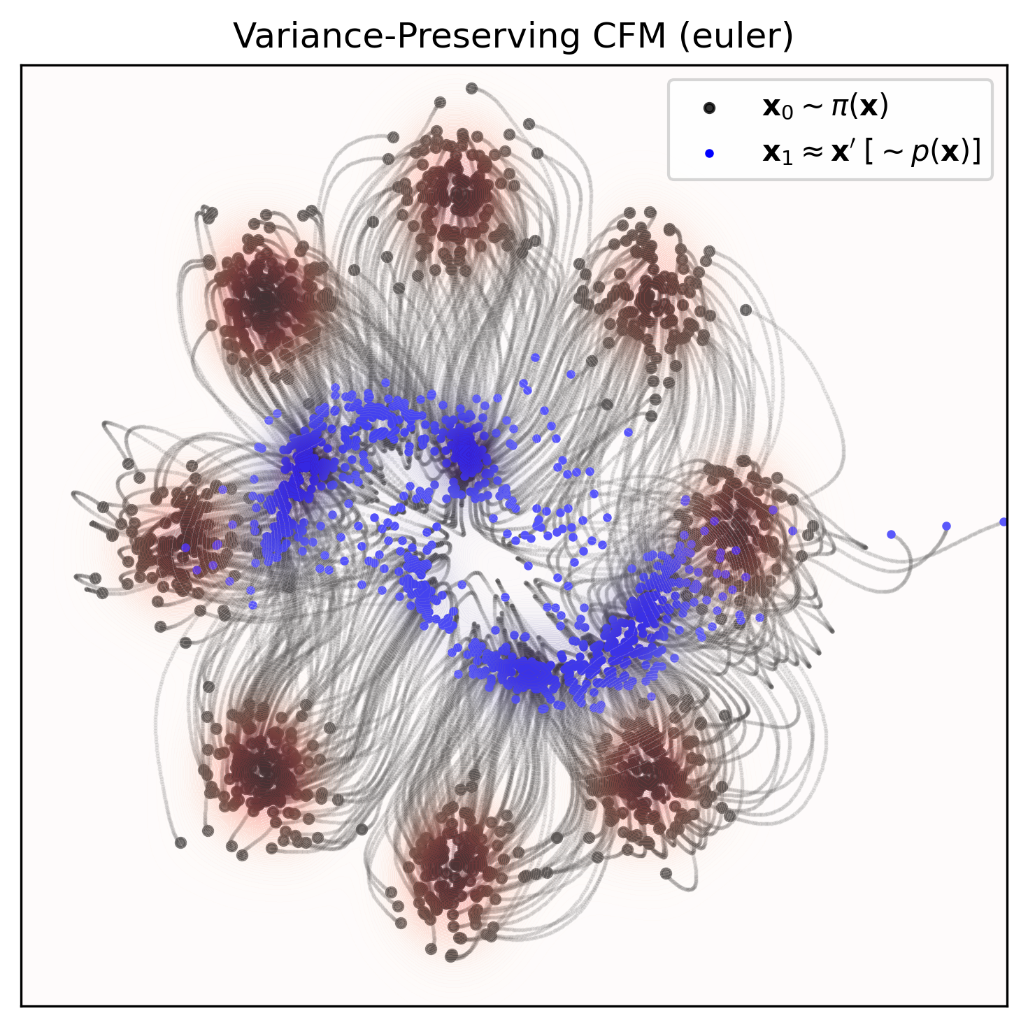
Conditional Flow Matching with ODE Solvers

Conditional Flow Matching (CFM): a simulation-free training objective for continuous normalizing flows.​ We explore a few different flow matching variants and ODE solvers on a simple dataset. This blog is a brief overview of the mlx-cfm GitHub repo, for simple conditional flow matching in MLX with ODE solvers.

Background

Training: consider a smooth time-varying vector field $u\,:\,[0, 1] \times \mathbb{R}^d \to \mathbb{R}^d$ that governs the dynamics of an ordinary differential equation (ODE), $dx = u_t(x)\,dt$. The probability path $p_t(x)$ can be generated by transporting mass along the vector field $u_t(x)$ between distributions over time, following the continuity equation

$$\frac{\partial p}{\partial t} = -\nabla \cdot (p_t u_t).$$

However, the target distributions $p_t(x)$ and the vector field $u_t(x)$ are intractable in practice. Therefore, we assume the probability path can be expressed as a marginal over latent variables:

$$p_t(x) = \int p_t(x | z) q(z)\, dz,$$

where $p_t(x | z) = \mathcal{N}\left(x | \mu_t(z), \sigma_t^2 I\right)$ is the conditional probability path, with a latent $z$ sampled from a prior distribution $q(z)$. The dynamics of the conditional probability path are now governed by a conditional vector field $u_t(x | z)$. We approximate this using a neural network, parameterizing the time-dependent vector field $v_\theta\,:\,[0,1] \times \mathbb{R}^d \to \mathbb{R}^d$. We train the network by regressing the conditional flow matching loss:

$$L_{\text{CFM}}(\theta) = \mathrm{E}_{t, q(z), p_t(x | z)} \lVert v_\theta(t, x) - u_t(x | z) \rVert^2,$$

such that $t \sim U(0,1), \; z \sim q(z), \; \text{and} \; x_t \sim p_t(x|z)$. But, how do we compute $u_t(x|z)$? Well, assuming a Gaussian probability path, we have a unique vector field (Theorem 3; Lipman et al. 2023) given by,

$$u_t(x | z) = \frac{\dot{\sigma}_t (z)}{\sigma_t (z)}\,\left(x - \mu_t(z)\right) + \dot{\mu}_t(z),$$

where $\dot{\mu}$ and $\dot{\sigma}$ are the time derivatives of the mean and standard deviation. If we consider $\mathbf{z} \equiv (\mathbf{x}_0, \mathbf{x}_1)$ and $q(z) = q_0(x_0)q_1(x_1)$ with

$$\begin{align} \mu_t(z) &= tx_1 + (1 - t) x_0, \\ \sigma_t(z) &= \sigma_{> 0}, \end{align}$$

then we have independent conditional flow matching (Tong et al. 2023) with the resulting conditional probability path and vector field

$$\begin{align} p_t(x | z) &= \mathcal{N}\left(x | tx_1 + (1 - t) x_0, \sigma^2\right), \\ u_t(x | z) &= x_1 - x_0. \end{align}$$

Alternatively, the variance-preserving stochastic interpolant (Albergo & Vanden-Eijnden 2023) has the form

$$\begin{align} \mu_t(z) = \cos \left(\pi t / 2\right)x_0 + \sin \left(\pi t / 2 \right)x_1 \quad\text{and}\quad \sigma_t(z) = 0,\\ u_t(x | z) = \frac{\pi}{2} \left( \cos\left(\pi t / 2\right) x_1 - \sin\left(\pi t / 2\right) x_0 \right). \end{align}$$

Sampling: now that we have our vector field, we can sample from our prior $\mathbf{x} \sim q_0(\mathbf{x})$, and run a forward ODE solver (e.g., fixed Euler or higher-order, adaptive Dormand–Prince) generally defined by

$$\mathbf{x}_{t+\Delta} = \mathbf{x}_{t} + v_\theta (t, \mathbf{x}_t) \Delta,$$

for $t$ steps between $0$ and $1$.

Getting Started

Check out the repo on GitHub to recreate the figure at the top of this post! 😄